Robert M. Powell, Powell & Associates Science Services
This page describes ground water sampling impacts on sample quality and how to resolve issues caused by the impacts.

Part 1. Sampling of Ground Water Monitoring Wells
Part 2. Sampling of Ground Water Monitoring Wells, Part 2 - Hydrogeologic Effects on Contaminants
Part 3. Sampling of Ground Water Monitoring Wells, Part 3 - Low-Flow and Passive Purging and Sampling

Download a Powell & Associates Science Services Draft Low-Flow Rate Purging and Sampling SOP:
SOP_DRAFT_Low-Flow

Sampling of Ground Water Monitoring Wells, Part 1-Turbidity Effects on Contaminant Concentrations in Samples

Many of the common ground water sampling techniques and procedures have resulted from methods developed for water supply investigations. These methods have persisted, even though the monitoring goals may have changed from water supply development to contaminant source and plume delineation. Unfortunately, the use of these methods can result in an incorrect understanding of the contaminant concentrations and system geochemistry, often overestimating or underestimating the true values or the extent of a plume. This article, and those following in the subsequent two issues, will attempt to explain why this occurs and how to sample in a manner that provides better data.

Ground water quality is typically determined by analyzing samples acquired from cased monitoring wells. Traditionally, three to five casing volumes of water are purged from each well prior to sample acquisition, typically at high pump rates or with a bailer. This is intended to remove stagnant casing water from the borehole, replacing it with water from the aquifer. Samples are then obtained in much the same manner, i.e by bailing or high-speed pumping. This approach to purging and sampling may seem reasonable, but numerous problems can occur that affect both sample quality and data interpretation.

It was discovered, during investigations of potential contaminant transport by mobile colloidal particles, that traditional purging and sampling were disrupting the aquifer and sand pack materials. The disruption was caused by the stress of high water velocities and/or water surging in the wells due to sampling with bailers and high-speed submersible pumps. This left no conclusive way to determine whether collected particulates in the samples were naturally occurring or due to the disturbance caused by the sampling device/approach.

Such induced stresses can cause grain flow within the sand pack and/or exceed the cohesive forces of aquifer mineral cementation, resulting in excessive and artificial sample turbidity. This increased turbidity can radically alter analytical results for water samples, causing spurious increases in analyzed metal concentrations. This is particularly true for the major constituents of the aquifer mineral matrix, such as iron, aluminum, calcium, magnesium, manganese, and silicon. Therefore, it has become standard practice for metals samples to be filtered through 0.45 µM pore-diameter filters to eliminate turbidity. This is the classical analytical definition of "dissolved" metals.

Unfortunately, colloidal particles are often smaller than 0.45 µM and can pass through the filter but cannot be considered "dissolved" for site transport modeling, risk assessment, or geochemical understanding. Such particles may or may not be naturally mobile in the aquifer. In addition, particles larger than 0.45 µM can be mobile in subsurface systems and may carry adsorbed contaminant species. These will be filtered out. Therefore, using the 0.45 µM filtration criterion, estimates of the contaminants in an aquifer may be either too high or too low, depending on a complex interrelationship between geophysical and geochemical conditions. This degree of complexity has arisen without even considering that the mean particle exclusion size of the filter can change during the course of the filtration due to filter pore plugging and blockage as excluded particles accumulate on and in the filter.

The collection and analysis of both filtered and unfiltered samples is sometimes suggested, but this data cannot resolve either the dissolved or colloidal contaminant concentrations. There is no way to know which, if either of the samples, accurately represents anything following the artificial particle entrainment, whether filtered or not. When aquifer/sand pack disruption occurs, fresh, reactive mineral particle surfaces are exposed to the aqueous solution. This provides a potentially very large surface area of reactive adsorption sites to bind the dissolved contaminants of interest. When the samples are filtered to remove the particles, the bound contaminants will also be removed. It is also possible that the disruption can release contaminants that were previously bound to, or incorporated within, the aquifer mineral matrix and were previously immobile and of no concern to human health and the environment. This release would yield artificially high contaminant values.

These considerations make it important to develop sampling methods that do not disrupt the aquifer matrix or sand pack and eliminate the need for filtration. Once artificial sample turbidity has occurred, there is no filtration method or sample treatment that can restore confidence in the data quality.

Sampling of Ground Water Monitoring Wells, Part 2-Hydrogeologic Effects on Contaminants

 In Part 1 of this series it was shown that traditional sampling techniques can adversely affect the quality of collected samples due to the entrainment of artificially generated turbidity. The following explains how hydrogeologic effects can also occur and confound our understanding of the true contaminant distributions and concentrations, and illustrates these effects with simple graphical examples.

Mixing of contaminated with uncontaminated waters in both the subsurface and in a monitoring well can occur when purging and sampling are improperly performed. This problem increases with longer well screens, higher pump rates, bailing, and when variable stratigraphy exists across the screened interval.

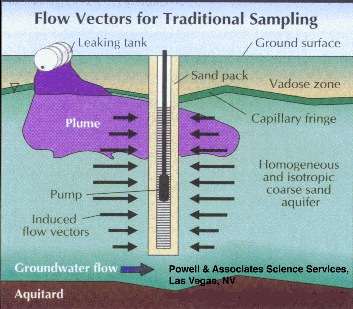
Long well screens tend to average the contaminant concentration over the vertical screen dimension, i. e. over the screen length. This is because traditional sampling techniques simultaneously pull water from all zones, both contaminated and uncontaminated, that the screen intersects (Figure 1). This may be satisfactory if the desired result is a concentration integrated over a fairly large volume of the aquifer. It yields little information, however, about plume thickness or contaminant concentration gradients within the actual plume.

Part 2, Figure 1. Long well screens tend to average the contaminant concentration over the vertical

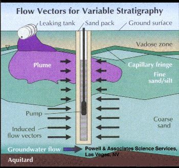
This problem can be worsened by stratigraphic variations that result in zones of high natural ground water flow layered with less permeable zones across the screened interval. In this situation, the water is preferentially transferred into the well casing from the higher permeability flow zones, whether or not these are the zones of maximum contamination (Figure 2).

Part 2, Figure 2. Preferential transfer of water from high permeability stratigraphy into long well screen.

High pump rates, can also yield false plume locations and higher-than-actual contaminant concentrations, especially when combined with the above long-screen scenarios. Figures 1 and 2 illustrate that wells with long screens can provide incorrect, low contaminant values but a potential overestimation of plume thickness. Figure 3 shows the potential for high pump rates to pull contaminated water into a zone where there previously was none. The figure depicts this occurrence via high-permeability sand, but fractured rock could also be very susceptible to such errors. This scenario results in overestimation of the natural extent of the plume as well as spreading of the contamination into uncontaminated zones. Although horizontally­induced migration is depicted, field data has shown that vertically­induced migration through the aquifer is also possible.

Part 2, Figure 3. False plume migration induced by high pumping rates.

Ideally, the screened interval should encompass only the sampling zone of interest, i. e. no more than the maximum vertical integration length that allows adequate characterization of the plume location and contaminant concentrations. The determination of what constitutes an adequate degree of characterization depends, of course, on the goals of the monitoring program. In general, pump rates should be set to attain only waters from the zones of interest and minimize induced hydrodynamic effects.

Figure 4 depicts such a sampling scheme. In this nested well scheme there are separate sampling points, with no sandpacks, and the aquifer has been allowed to collapse around the sampling point. These can be installed with small diameter augers or with the use of drive-point technologies. These types of monitoring points are probably best sampled through low-flow purging and sampling techniques, with the monitoring of purging parameters such as turbidity, Eh, and DO. It is also possible to sample such monitoring wells using passive, or unpurged sampling, depending on natural ground water flow to maintain purged conditions.

Part 2, Figure 4. Nested multilevel downgradient sampling wells with discrete sampling intervals and no sandpacks.

Sampling of Ground Water Monitoring Wells, Part 3-Low-Flow and Passive Purging and Sampling

In the first two installments of this series, the problems of induced turbidity and hydrodynamic mixing of contaminated and uncontaminated ground waters during sampling were discussed. An additional concern is the disposal of large volumes of purged water that must be handled and treated as hazardous waste. These problems can often be minimized by using lower flow rates and greater care during sample collection.

Studies have shown that groundwater in the screened interval of a standard monitoring well can be representative of that in the formation, even though stagnant water lies above in the casing. This occurs when flow is generally horizontal and naturally purges the screened interval (Figure 5). Unfortunately, the insertion of a sampling device, such as a pump, bailer, or even a tube can disrupt this equilibrium and cause mixing of the screened and cased interval waters (Figure 6). The mixture of stagnant and screened interval water can even potentially be forced into the aquifer in all directions, including upgradient. This can result in unpredictable geochemical and microbiological effects that may effect data quality from the well over the short, and possibly long term.

Part 3, Figure 5. Natural purging of the screened interval of a monitoring well by horizontal ground water flow.


Part 3, Figure 6. Disruption of horizontal ground water flow by insertion of a sampling device, causing mixing of stagnant casing waters with the screened interval waters.

Following device insertion, some amount of time must elapse before the equilibrium of Figure 5 is reestablished. Therefore, both low-flow and passive sampling techniques are most accurate using dedicated sampling devices that can be left down-hole. Alternatively, if devices cannot be dedicated, the sampling devices can be slowly and carefully inserted and left until the screen/casing equilibrium returns or is approximated. This allows a pump, for example, to be used in multiple wells, but requires additional time and planning. Both these approaches minimize, and potentially eliminate purge time and volume.

Possibly less accurate, but still typically yielding data superior to high-flow techniques, is careful device insertion followed immediately by low-flow purging and sampling.

Low-Flow Purging and Sampling

This method of sampling is now well documented and becoming widely adopted. It consists basically of only a few modifications to traditional techniques that sample ground water with pumps.

The pump inlet is placed in the screened interval at the point where the contaminant concentration is desired (but not at the very bottom of the borehole due to the accumulation of solids in this region). Usually the desired location is the zone of highest contaminant concentration. Short screened intervals across this zone are desirable for the reasons discussed in Part 2 of this series. Purging is then begun, typically at a rate of 0.1 to 0.5 L/min, although rates up to 1 L/min may be allowable in highly transmissive formations.

During the course of purging, certain parameters should be tracked to determine when they become reasonably stable, indicating sampling continuity with the formation water. If possible, these parameters should be measured directly in the flow stream very near the well head to eliminate atmospheric exposure and temperature changes. Traditionally, pH, temperature and conductivity have been used as these parameters. Temperature and pH have been shown to be insensitive, however, relative to DO, Eh, and turbidity. Whenever possible, the concentration of the contaminant(s) of interest should also be tracked for stability. The parameters are usually considered stable when 3 consecutive readings within ± 10% of one another for DO and turbidity (or ± 10 mV for Eh) are obtained over a 3 to 10 minute period. At that time samples are acquired, typically unfiltered due to the reasons discussed in Part 1 of this series.

Passive Sampling

Passive sampling requires stabilized well conditions, as previously discussed, but generates the lowest purge volume of any of the sampling techniques. Used properly, it also has the potential for providing the best contaminant concentration data. The most accurate data is likely to be obtained from small diameter (e.g. d < 2 inch) wells without sand packs, with short (e.g. one foot or less) screened intervals placed directly in the zones of interest. Often these wells are nested to allow sampling of multiple depths at the same surface location. When the sampling depth is within suction lift range, peristaltic pumps have been shown to work well for inorganics, although volatile organic constituents may be somewhat biased to lower than actual values. At greater depths, or for the most accurate determinations of volatile organic compounds, low-speed submersible and bladder pumps can be used.

One goal of passive sampling is to obtain the needed samples with the minimum possible disturbance to the water in the well. Increased disturbance translates to increased purging volume and time. With dedicated samplers and passive sampling techniques, the only purging required is to evacuate the sampling device (pump body, tubing, etc.) itself.

A typical passive-sampling scenario can be as simple as:

1. Adjust the pump/controller to the proper (slow) sampling speed and turn it off.
2. Attach the pump/controller to the tubing exiting the well and start the pump.
3. Purge enough water to remove the sampling device volume at least once (two to three times might be preferable but the risk of acquiring stagnant casing water increases with each device volume removed, especially when sampling a non-transmissive formation).
4. Collect and preserve the samples.
5. Measure the water level (Note: this step should always follow the sampling when using passive techniques, to avoid initial disturbance to the stagnant water).
6. Close up and proceed to the next well.

 
The "slow" pump rate referred to in this procedure is far slower than typically used. A suggested range could be somewhere between 10 to 100 ml/min, depending somewhat on the hydraulic characteristics of the screened interval and the natural pore water velocity in that zone, as well as limitations of the sampling device.

When using passive sampling techniques it is not always necessary to track indicator parameters for aquifer water continuity, as presented in the previous section on low-flow purging and sampling. However, it is a good idea to document these parameters the first few times a well is sampled. This will, of course, require additional purging during the documentation period. It also requires that the sampling device has been downhole for a period sufficient allow the well equilibrium (Figure 5) to become re-established before the test begins. If the changes in parameter values after the sampling device purge volumes are withdrawn are insignificant, then passive sampling is justifiable because additional purging makes no difference. If significant changes in the parameter readings do occur, the interpretation becomes more difficult. In this case a decision must be made as to which of the sampling methodologies is giving the more accurate values. The more conservative approach would be to choose the method that yields the higher contaminant values.

A potential method for resolving such discrepancies is the use of data from a Geoprobe®, HydroPunch® or other similar push tool technology (provided the push samples have been taken in the same three-dimensional location as the current well emplacement). This may not be considered practical for older monitoring wells but, increasingly, the locations of new monitoring wells and screened intervals are being based on such data.